Creating Functions

Overview

Teaching: 30 min
Exercises: 0 min

Questions

How can I teach MATLAB how to do new things?

Objectives

Compare and contrast MATLAB function files with MATLAB scripts.

Define a function that takes arguments.

Test a function.

Recognize why we should divide programs into small, single-purpose functions.

If we only had one data set to analyze, it would probably be faster to load the file into a spreadsheet and use that to plot some simple statistics. But we have twelve files to check, and may have more in future. In this lesson, we’ll learn how to write a function so that we can repeat several operations with a single command.

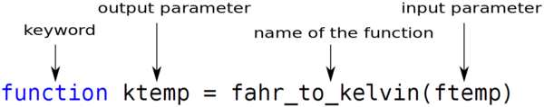
Let’s start by defining a function fahr_to_kelvin that converts temperatures from Fahrenheit to Kelvin:

function ktemp = fahr_to_kelvin(ftemp)
    %FAHR_TO_KELVIN   Convert Fahrenheit to Kelvin

    ktemp = ((ftemp - 32) * (5/9)) + 273.15;
end

A MATLAB function must be saved in a text file with a .m extension. The name of that file must be the same as the function defined inside it. The name must start with a letter and cannot contain spaces. So, you will need to save the above code in a file called fahr_to_kelvin.m. Remember to save your m-files in the current directory.

The first line of our function is called the function definition, and it declares that we’re writing a function named fahr_to_kelvin, that has a single input parameter,ftemp, and a single output parameter, ktemp. Anything following the function definition line is called the body of the function. The keyword end marks the end of the function body, and the function won’t know about any code after end.

function-definition

A function can have multiple input and output parameters if required, but isn’t required to have any of either. The general form of a function is shown in the pseudo-code below:

function [out1, out2] = function_name(in1, in2)
    %FUNCTION_NAME   Function description

    % This section below is called the body of the function
    out1 = something calculated;
    out2 = something else;
end

Just as we saw with scripts, functions must be visible to MATLAB, i.e., a file containing a function has to be placed in a directory that MATLAB knows about. The most convenient of those directories is the current working directory.

GNU Octave

In common with MATLAB, Octave searches the current working directory and the path for functions called from the command line.

We can call our function from the command line like any other MATLAB function:

>> fahr_to_kelvin(32)

ans = 273.15

When we pass a value, like 32, to the function, the value is assigned to the variable ftemp so that it can be used inside the function. If we want to return a value from the function, we must assign that value to a variable named ktemp—in the first line of our function, we promised that the output of our function would be named ktemp.

Outside of the function, the variables ftemp and ktemp aren’t visible; they are only used by the function body to refer to the input and output values.

This is one of the major differences between scripts and functions: a script can be thought of as automating the command line, with full access to all variables in the base workspace, whereas a function can only read and write variables from the calling workspace if they are passed as arguments — i.e. a function has its own separate workspace.

Now that we’ve seen how to convert Fahrenheit to Kelvin, it’s easy to convert Kelvin to Celsius.

function ctemp = kelvin_to_celsius(ktemp)
    %KELVIN_TO_CELSIUS   Convert from Kelvin to Celcius

    ctemp = ktemp - 273.15;
end

Again, we can call this function like any other:

>> kelvin_to_celsius(0.0)

ans = -273.15

What about converting Fahrenheit to Celsius? We could write out the formula, but we don’t need to. Instead, we can compose the two functions we have already created:

function ctemp = fahr_to_celsius(ftemp)
    %FAHR_TO_CELSIUS   Convert Fahrenheit to Celcius

    ktemp = fahr_to_kelvin(ftemp);
    ctemp = kelvin_to_celsius(ktemp);
end

Calling this function,

>> fahr_to_celsius(32.0)

we get, as expected:

ans = 0

This is our first taste of how larger programs are built: we define basic operations, then combine them in ever-larger chunks to get the effect we want. Real-life functions will usually be larger than the ones shown here—typically half a dozen to a few dozen lines—but they shouldn’t ever be much longer than that, or the next person who reads it won’t be able to understand what’s going on.

Concatenating in a Function

In MATLAB, we concatenate strings by putting them into an array or using the strcat function:
>> disp(['abra', 'cad', 'abra'])
abracadabra
>> disp(strcat('a', 'b'))
ab
Write a function called fence that has two parameters, original and wrapper and adds wrapper before and after original:
>> disp(fence('name', '*'))
*name*
Solution
function wrapped = fence(original, wrapper)
    %FENCE   Return original string, with wrapper prepended and appended

    wrapped = strcat(wrapper, original, wrapper);
end

Getting the Outside

If the variable s refers to a string, then s(1) is the string’s first character and s(end) is its last. Write a function called outer that returns a string made up of just the first and last characters of its input:
>> disp(outer('helium'))
hm
Solution
function ends = outer(s)
    %OUTER   Return first and last characters from a string

    ends = strcat(s(1), s(end));
end

Variables Inside and Outside Functions

Consider our function fahr_to_kelvin from earlier in the episode:
function ktemp = fahr_to_kelvin(ftemp)
  %FAHR_TO_KELVIN   Convert Fahrenheit to Kelvin
  ktemp = ((ftemp-32)*(5.0/9.0)) + 273.15;
end
What does the following code display when run — and why?
ftemp = 0
ktemp = 0

disp(fahr_to_kelvin(8))
disp(fahr_to_kelvin(41))
disp(fahr_to_kelvin(32))

disp(ktemp)
Solution
259.8167
278.1500
273.1500
0
ktemp is 0 because the function fahr_to_kelvin has no knowledge of the variable ktemp which exists outside of the function.

Testing a Function

Write a function called normalise that takes an array as input and returns an array of the same shape with its values scaled to lie in the range 0.0 to 1.0. (If L and H are the lowest and highest values in the input array, respectively, then the function should map a value v to (v - L)/(H - L).) Be sure to give the function a comment block explaining its use.

Run help linspace to see how to use linspace to generate regularly-spaced values. Use arrays like this to test your normalise function.
Solution
function out = normalise(in)
    %NORMALISE   Return original array, normalised so that the
    %            new values lie in the range 0 to 1.

    H = max(max(in));
    L = min(min(in));
    out = (in-L)/(H-L);
end
a = linspace(1, 10);   % Create evenly-spaced vector
norm_a = normalise(a); % Normalise vector
plot(a, norm_a)        % Visually check normalisation

Convert a script into a function

Convert the script from the previous episode into a function called analyze_dataset. The function should operate on a single data file, and should have one parameter: file_name. When called, the function should create the three graphs produced in the previous lesson. i.e. analyze_dataset('inflammation-01.csv') should save the figures for the first dataset to the results directory.

Be sure to give your function help text.

function analyze_dataset(file_name)
    %ANALYZE_DATASET    Perform analysis for named data file.
    %   Create figures to show average inflammation.
    %
    %   Example:
    %       analyze_dataset('data/inflammation-01.csv')
    
    % Generate string for image name:
    img_name = replace(file_name, 'inflammation', 'patient_data');
    img_name = replace(img_name, '.csv', '.png');
    img_name = fullfile('results', img_name);
    patient_data = csvread(file_name);
    
   	figure('visible', 'off')
    
    plot(mean(patient_data, 1))
    title('Daily average inflammation')
    xlabel('Day of trial')
    ylabel('Inflammation')
    
    print('-dpng', img_name)
    
    close()
    
end

Automate the analysis for all files

Write a script called process_all which loops over all of the data files, and calls the function analyze_dataset for each file in turn.

 %PROCESS_ALL    Analyse all inflammation datasets
 %   Create figures to show average inflammation.
 %   Save figures to 'results' directory.

 files = dir('data/inflammation-*.csv');

 for i = 1:length(files)
     file_name = files(i).name;

     % Process each data set, saving figures to disk.
     analyze_dataset(file_name);
 end

We have now solved our original problem: we can analyze any number of data files with a single command. More importantly, we have met two of the most important ideas in programming:

Use arrays to store related values, and loops to repeat operations on them.
Use functions to make code easier to re-use and easier to understand.

Key Points

Break programs up into short, single-purpose functions with meaningful names.

Define functions using the function keyword.

previous episode

Programming with MATLAB

next episode

Creating Functions

Overview

GNU Octave

Concatenating in a Function

Solution

Getting the Outside

Solution

Variables Inside and Outside Functions

Solution

Testing a Function

Solution

Convert a script into a function

Automate the analysis for all files

Key Points

previous episode

next episode